Refinamento da estimativa de retorno de mercado esperado: fundindo vários modelos de avaliação de empresas como uma abordagem para reduzir a incerteza

Thiago Petchak Gomes [1]

 

ABSTRACT

This paper presents a methodology aimed at reducing the uncertainty associated with estimating the expected market return within a bounded rationality framework. The proposed approach involves calculating the implicit rate of return using various valuation models and subsequently merging them using the Kalman Filter technique to minimize estimation errors. The contribution of this study lies in the application of the Kalman Filter, which enables the expected market return to be refined and provides a more accurate estimate by mitigating uncertainty. The ability to determine an accurately expected market return assumes critical significance in investment decision-making. Therefore, investors can utilize this methodology as a tool to enhance the precision of their investment choices. By reducing uncertainty in estimating the expected market return, this approach empowers investors to make more informed and confident decisions.   

Keywords: Kalman Filter; Valuation models; Uncertainty; Market Expected Return.

 

RESUMO

Este artigo apresenta uma metodologia que visa reduzir a incerteza associada à estimativa dos retornos esperados do mercado em um quadro de racionalidade limitada. A abordagem proposta envolve o cálculo da taxa de retorno implícita utilizando vários modelos de precificação de ativos e posteriormente fundindo-os utilizando a técnica do Filtro de Kalman para minimizar erros de estimativas. A contribuição deste estudo é a aplicação do Filtro de Kalman, que permite refinar o retorno esperado do mercado e fornece uma estimativa mais precisa ao mitigar a incerteza. A capacidade de determinar com melhor precisão um retorno de mercado esperado assume importância crítica na tomada de decisões de investimento. Portanto, os investidores podem utilizar esta metodologia como uma ferramenta para aumentar a precisão das suas escolhas de investimento. Ao reduzir a incerteza na estimativa dos retornos esperados do mercado, esta abordagem permite que os investidores tomem decisões mais informadas e confiantes. 

Palavras-chave: Filtro de Kalman; modelos de precificação de ativos; incerteza; retorno esperado de mercado

 1. Introduction

Defining a reasonably accurate expected market return can be a crucial element between accepting or rejecting an investment. In other words, when applying the Capital Asset Pricing Model – CAPM, proposed by Sharpe (1964), as a tool to estimate the cost of equity for a potential project, the expected net present value of a project's cash flows can be negative or positive, simply depending on the parameters applied in CAPM. A survey carried out by Martelanc, Trizi, Pacheco, and Pasin between March and November 2004 with 29 M&A and private equity professionals working in Brazil's leading investment banks and financial advisors showed that the main method used to determine the market risk premium is the historical average of that variable. Despite this, Elton (1999) believes that “there is ample evidence that using realized returns as a proxy for expected returns is wrong.” Elton (1999) points out that “there are periods [in the United States] greater than 10 years which stock market realized returns are, on average, lower than the risk-free rate (1973 to 1984) and periods greater than 50 years in which risky long-term bonds underperform the risk-free rate (1927 to 1981).” Applying a market risk to the CAPM that is lower than the risk-free rate is wrong: it would say that the market is less risky than the risk-free rate. In other words, this fact would result in a negative slope market line, neglecting the risk and return tradeoff suggested by Markowitz in 1952. Furthermore, using the historical average return as a proxy for market return can have some problems even during the periods in which these returns exceed the risk-free rate. For Sanvicente and Carvallho (2020), "the use of the historical return is in strong conflict with the concept of opportunity cost: for an individual or a company that needs to make an investment decision, the relevant cost must be that prevailing at the moment the decision must be made, not an average of what has occurred in the past.”

As an alternative to the application of the historical return, Elton (1999) suggests the use of the implicit stock returns’ average. Sanvicente and Carvallho (2020), following Elton's (1999) proposal, used the dividend perpetuity model suggested by Gordon (1959) to calculate the implicit return. In this study, Sanvicente and Carvallho (2020) pointed out that the expected market return could be obtained from the average of the implicit return of all stocks traded on B3, following the dividend perpetuity model.

Besides the dividend perpetuity model, I believe that many other valuation models could be used to calculate the market expected return, which may result in different values, as well as different measurements’ uncertainties. In section 2, it will be presented a couple of alternative valuation models and in section 3 their respective implicit return equations. 

In this study, the valuation models’ measurements’ uncertainties will be related to Simon’s bounded rationality concept (1947). Although the CAPM states as a premise that all investors have the same expectations about the assets’ return, as a consequence of perfect information availability, given the bounded rationality concept, there is an incompleteness of information (Simon 1947). Cyert and March (2013), in line with Simon (1947), state that information is scarce, which results in an uncertain environment. Cristofaro (2017) asserts that “as a cumulative effect of bounded rationality, people make “satisficing” rather than “optimal” decisions. Therefore, this paper will show a method that reduces as much as possible (but not fully eliminate) the uncertainty of the market expected return estimation, considering a scenario with a lack of information. 

It’s important to state that, according to ABNT ISO/IEC Guia 98-3, the result of any value measurement is only an approximation or estimation of the measured value, thus, the measurement is only complete when it is accompanied by its uncertainty. Complementarily, about the measurement’s methods, ISO 5725 differs the terms trueness and precision. Applying ISO 5725 definition to this study, trueness will be related to the closeness between the estimated values to the adjusted realized market return, while precision is the closeness between the market expected return values that each valuation model indicates. Figure 1 illustrates the difference between trueness and precision. For this study, uncertainty will be related to a lack of trueness and precision: in section 3 of this paper, it will be shown in more detail the difference between those two terms.

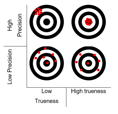
Figure 1 - Trueness and precision illustration

Under a noisy environment, with independent estimation errors that follow a Gaussian distribution, the Kalman Filter may provide the solution that estimates the best value of a given uncertain variable (Wells 1996). In addition, Wells (1996) points out that the term “best” should be interpreted as the minimum mean square estimator (MMSE) as the state vector itself is stochastic.” In this case, the uncertainty cannot be fully eliminated, but it can be reduced. Section 4 shows the Kalman Filter with more details and also why and how it can be applied for this study.

Therefore, considering the implicit return method as an approach to determine the expected market return and, also, that many valuation models can be used to calculate the market expected return – which may result in different values and uncertainties – this study aims to propose a method that combines different valuation models, by applying the Kalman Filter technique, as a way to determine the least uncertain possible value for market expected return (by maximizing the trueness and precision of the estimators).

This paper will be presented as follows: Section 2 presents some valuation models that can be used in the proposed approach; section 3 presents how to calculate the market expected return from the implicit return approach, and its respective trueness and precision; section 4 presents a method that combines the different valuation models, by applying the Kalman Filter technique, to reduce the uncertainty (maximizing precision and accuracy); and section 5 concludes it.

2. Valuation Models 

The purpose of this chapter is to briefly show a few (but not all) valuation models that are presented in the financial literature. Then, the implicit market return of each valuation model will be combined using the Kalman Filter, to reduce the uncertainty of market expected, as mentioned: which steps will be shown in the following sections. 

2.1 Gordon Dividend’s Perpetuity Formula 

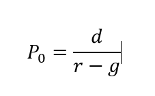
The dividend perpetuity formula proposed by Gordon and Shapiro (1956) suggests that the price of a stock with constant growth equals to equation 1, in which  is the price of a stock,  is expected dividend,  is the cost of capital, and  the dividend perpetual growth:

(1)

2.2 Clean Surplus Valuation

The clean surplus valuation is a derivation of the dividend perpetuity formula (Dechow, Hutton and Sloan, 1999) as shown in equation 2, where  is the price of a stock,  are the earnings per share,  is the book value per share at period t,  is the book value per share at period t-1, and  is the rate of return. 

(2)

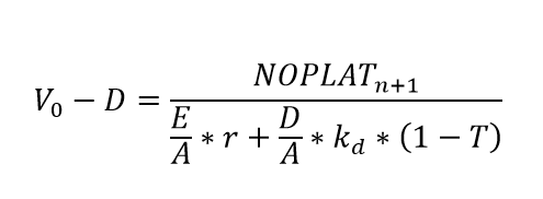
2.3 Copeland And Weston Value Formula (2014)

According to Copeland and Weston (2014) the value of a firm – which also includes the liabilities – is presented in equation 3, where V₀ is the value of the firm,  is the total debt,  is the net operating profit less adjusted taxes,  is the total equity,  is the total asset,  is the equity rate of return,  is the cost of debt and  is the tax rate:

 

(3)

2.4 Residual Income Valuation

The Residual Income Valuation Model was proposed by Ohlson (1995) as it is shown in equation 4, in which the  is the price of a stock,  is the book value at time t-1 divided by the number of shares,  is the return on equity, and  is the equity rate of return. 

 

(4)

2.5 Abnormal Earnings Growth 

The Abnormal Earnings Growth model was developed by Ohlson and Juettner-Nauroth (2005), which formula is shown in equation 5, where  are the earnings per share and  are the earnings per share at time t+1 plus the dividends per share at time t, minus the multiplication of the earnings per share at time t by .

 

(5)

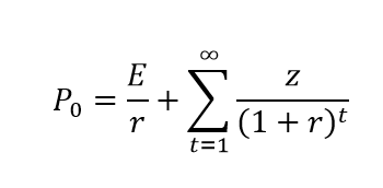
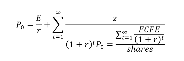
2.6 Discounted Cash Flow

The discounted cash flow valuation formula states that the price per share equals the net present value of the free cash flow to equity  (Kenton, 2021) divided by the number of shares, as shown in equation 6. 

 

(6)

  

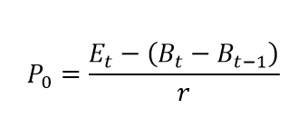
3. The Market Expected Return From The Implicit Rate Of Return Approach And Its Respective Trueness And Precision

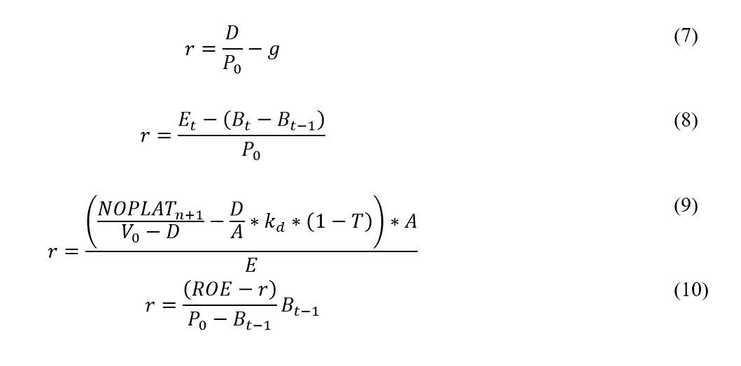
The first step to find the market expected return is to calculate the implicit rate of return for each asset, which, according to Elton (1999), is the discount rate that makes the net present value equal to zero. In other words, the implicit rate of return is the commonly known internal rate of return - IRR. Then, considering that the prices of the stocks are perfectly priced, the implicit rate of return from the valuation models presented in equations 1, 2, 3, and 4 of this paper are presented in equations 7, 8, 9, and 10, respectively. Although for equations 5 and 6 it is not possible to isolate the term r, it can be found by calculating the internal rate of return on any financial calculator. 

Taking into account a bounded rationality scenario, in which the agents do not have full information about the valuation models, it is expected that some parameters applied to the models presented in section 2 deviate from the actual value. In other words, the subjectivity needed to run the models cannot be fully eliminated. Thereat, as mentioned before, if those errors are independent, unbiased, and follow a gaussian distribution, it is expected that the Kalman Filter will reduce the estimation errors, resulting in a more accurate value compared to each model individually. Anyhow, to reduce even more (but still not eliminate) the models' uncertainty, it is recommended to do some refinements in the valuation parameters, such as the following two suggestions presented by Gordon (1959): 1) analyze the correlation between the variables and the variation in the coefficients between the industries; and 2) consider that the price of a share also varies with other variables, such as the size of the corporation, the relation of debt to equity and the stability of its earnings.

The next proposed step is to calculate the model uncertainty (lack of trueness and precision). It is expected that the realized return of a stock between period t-1 and t may equal to the expected return of that stock in period t-1, plus the sum of the sensitivity of the stock price to changes in macro factors' expectations – such as changes in inflation, GDP, and interest rate expectations –, multiplied by those factors’ variations between period t-1 and t plus an uncertainty, as shown in equation 11. 

 

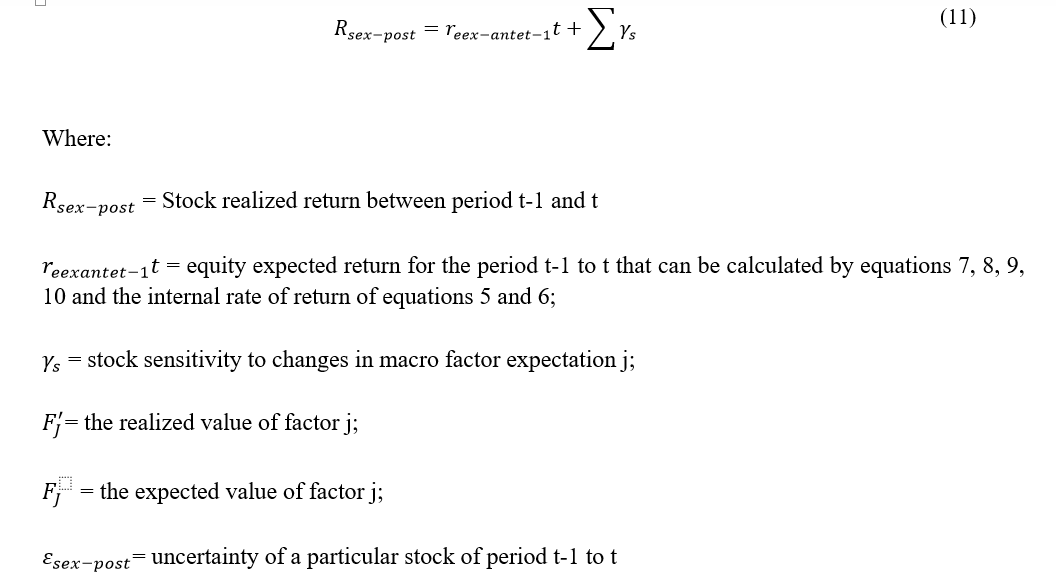
The reason to calculate the stock sensitivity to changes in macro factor expectations is that between period t-1 and t some market factors can simply vary from their expectation that could move the implicit risk either up or downward. The term  can be calculated by a regression model in which considers the historical price variation of a stock and market surprises   about macro factor variables. As it can be noted,  is simply the application of the Arbitrage Pricing Theory (APT) proposed by Ross in 1976. 

In addition, the term  of equation 11 can also be set as shown in equation 12: 

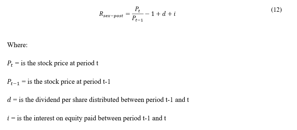
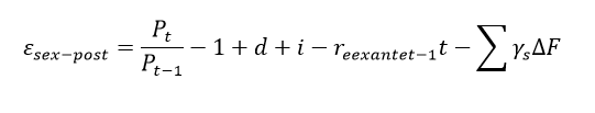
Then, equation 13 isolates the term of equation 11 and substitutes  to  of equation 12:

(13)

It is expected that the term   is related to the lack of trueness, lack of precision, and uncertainty caused by other factors not considered in the model. By the law of large numbers – considering the number of publicly traded companies – and since the APT aims to reduce the term , this work states as a premise that the uncertainty caused by other factors not considered in the model has a zero mean, and therefore, it can be neglected (which may not be necessarily true and needs to be better analyzed in future studies). 

The aggregation of all  for all publicly traded companies for a specific period in time, which  was calculated by a particular implicit expected return model, is expected to be normally distributed. The distance between that normally distributed curve mean to zero is related to the model's lack of trueness, as illustrated in figure 2. 

 

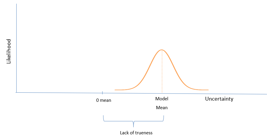
Figure 2 - Lack of trueness illustration

This study suggests that the lack of trueness can be corrected by shifting the curve of the ex-ante r_{m t to t+1} curve. So, for every  calculated from a certain valuation model from period t to t+1, it will be added or decreased the necessary amount that would shift the  to a zero mean. By doing that, it is expected that the part of uncertainty related to the lack of trueness to be reduced. That uncertainty may not be fully reduced, because the lack of trueness calculated between period t-1 to period t will not necessarily behave equally between period t to period t+1. Hence, future studies can develop a better way to solve that issue.

Considering that the lack of trueness has been decreased by using the suggested methodology in this study, the next step is to reduce the lack of precision. As mentioned, precision is the closeness between the market expected return values that each valuation model indicates

For all implied rates of return calculated of all publicly-traded companies from the different valuation models, the next step is to find the ex-ante market expected return, for period t to t+1, which can be calculated applying the Cost of Asset Pricing Model – CAPM (Sharpe, 1964 and Lintner, 1965). By calculating the companies’ beta – in other words: the companies’ sensitivities to market oscillations – and considering that the asset implicit rate of return equals to its asset’s expected rate of return, the market expected return can be found as shown in equation 14: 

It is important to note that there is no innovation in equation 9 from the CAPM model proposed by Sharpe (1964): there is only simple math where the market expected rate of return is isolated from the other terms. Also, under an unlimited rationality scenario, it would be expected that the market expected return calculated from any company and valuation model to be the same. However, given a bound rationality scenario, with noise and uncertainties, for any valuation model, it is expected to occur some variance for market expected return estimation (lack of precision). Just as an illustration, figure 1 shows how the ex-ante market expected returns from three different valuation models could behave for a given period in time. 

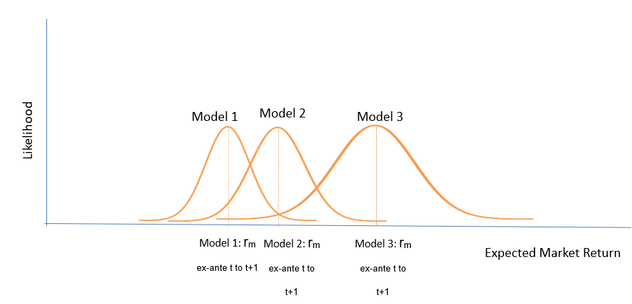
Figure 3 - Precision illustration

Given that precision is defined as the closeness between the market expected return values, if the market expected return calculated as shown in equation 10 is normally distributed, the precision for any valuation model can be set as the variance of its values. So, each model will have its estimated value for the expected market return, which is the model’s mean, and its respective variance. Also, this study suggests adding the term  multiplied by negative one to the ex-ante market expected return of each model, for period t to t+1. So, the ex-ante expected market return, of period t to t+1, for valuation model j added by the term  will be then called . In addition, the expected market variance for the valuation model j for the period t to t+1 will be then called . 

 4. The Kalman Filter

As a reminder, this study aims to reduce the uncertainty caused when is the market expected return is estimated. The reason for that is because, as mentioned, when applying the Capital Asset Pricing Model - CAPM as a tool to estimate the cost of equity for a potential project, the expected net present value of a project's cash flows can be negative or positive, simply depending on the parameters applied in CAPM. 

The Kalman Filter can be used as a tool to reduce the lack of precision caused by noise or other variables not considered in the valuation models, by minimizing the quadratic function of estimator error (Grewal and Andrews, 2014). According to Grewal and Andrews, 2014) “if one wants to very precise estimates of their characteristics over time, the one has to take their dynamics into consideration. The problem is that one those not always know their dynamics very precisely either. Given this state of partial ignorance, the best one can do is express our ignorance more precisely – using probabilities. The Kalman filter allows us to estimate the state of dynamics systems with certain types of random behavior by using statistical information.” By analyzing the characteristics of the problem presented in this paper, the Kalman Filter may be a useful tool to resolve that problem. 

Consider that for a certain period in time it has been calculated the values for  and  from three different valuation models using the implied return methodology. This study suggests that each value of , from each valuation model, can be viewed as a specific type of sensor that calculates the market expected return for a period. Also, its respective   is the noise of that sensor – in other words: its lack of precision. The values of  and  for a specific time will not necessarily be equal from one valuation model to another. Then, this paper recommends applying the Kalman Filter as a way to fuse those values, aiming to reduce as much as possible the lack of precision of the estimators. 

Therefore, by applying the Kalman Filter, the expected market return estimated from the fusion of different  will be called in this paper as , which can be calculated as shown in equation 15.

(15)

The term  is the ex-ante expected market return using, for example, equation 7 of this paper, while  is the ex-ante expected market return using, for example, equation 8. KG is the so-called Kalman Gain, which can be calculated by applying equation 16. 

 

(16)

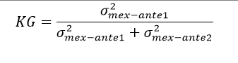
The term  is the ex-ante variance, of period t to t+1, calculated using any valuation model – for example, equation 7 –, while  is the ex-ante variance, of period t to t+1, calculated using the valuation model shown in equation 8, for example. If  is higher than , the Kalman Filter will give a higher weight on  than . Then, as closer KG is to 1, the most Kalman filter will rely on . On the other side, as closer KG is to 0, the most Kalman filter will rely on . 

The next step is to calculate the resulting variance after the interaction of  and . Based on Biezen (2015), the variance () of   can be calculated by the equation 17: 

(17)

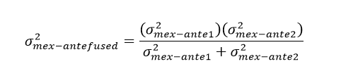
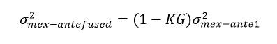
Also based on Biezen (2015), equation 17 can be expressed according to equation 18: 

(18)

5. Conclusion

Considering a bounded rationality scenario, the actual market expected return cannot be known without the presence of uncertainty. In order to reduce that uncertainty, this paper suggests fusing multiple valuation models, as a process of sensor fusion, using the Kalman Filter tool. By applying the Kalman Filter, it is expected that the expected market return will be moved to a more precise value, once the uncertainty is decreased. In addition, by adding more valuation models to the processes – once it is independent of the other models and normally distributed – the uncertainty of the market expected return estimation may be decreased. 

In order to complement this study, future empirical studies may be done to better analyze the robustness of the methodology proposed. Finally, future research may be done to figure out the determinants that cause the uncertainties variation from one period to another and its correlation to the market expected return, for example, to analyze if those variables are perfectly correlated through time, or if there are periods in which the market expected return and uncertainty move in opposite directions. 

Bibliography

ABNT ISO/IEC GUIA 98-3. Incerteza de Medição Parte 3: Guia para a expressão de Incerteza de medição (GUM:1995), 18. Dec. 2014.

ABNT NBR. ISO 5725-1 Accuracy (trueness and precision) of measurement method and results. 2018.

COPELAND, T. E.; J  FRED WESTON; SHASTRI, K. Financial theory, and corporate policy. 4th ed. Harlow: Pearson Education Limited, 2014.

CRISTOFARO, M. Herbert Simon’s bounded rationality. Journal of Management History, v. 23, n. 2, p. 170–190, 2017.

DECHOW, P. M.; HUTTON, A. P.; SLOAN, R. G. An empirical assessment of the residual income valuation model. Journal of Accounting and Economics, v. 26, n. 1-3, p. 1–34, 1999.

ELTON, E. J. Presidential Address: Expected Return, Realized Return, and Asset Pricing Tests. The Journal of Finance, v. 54, n. 4, p. 1199–1220, 1999. Acesso em: 29/1/2022.

GORDON, M. J. Dividends, Earnings, and Stock Prices. The Review of Economics and Statistics, v. 41, n. 2, p. 99, 1959.

GORDON, M. J.; SHAPIRO, E. Capital Equipment Analysis: The Required Rate of Profit. Management Science, v. 3, n. 1, p. 102–110, 1956. Acesso em: 29/1/2022.

GREWAL, M. S.; ANDREWS, A. P. Kalman filtering theory and practice using MATLAB. 4th ed. Hoboken, Nj Wiley, 2015.

KENTON, W. Understanding Free Cash Flow to Equity. Disponível em: <https://www.investopedia.com/terms/f/freecashflowtoequity.asp>. Acesso em: 30/1/2022.

MARKOWITZ, H. Portfolio Selection. The Journal of Finance, v. 7, n. 1, p. 77–91, 1952.

MERTELANC, R., TRIZI, J. S., PACHECO, A. S. Metodologias de Avaliação de Empresas: Resultados de uma pesquisa no Brasil, 2004.  

MICHEL VAN, B. Special Topics - The Kalman Filter (3 of 55) The Kalman Gain: A Closer Look. Disponível em: <https://www.youtube.com/watch?v=fpRb1sjFz_M&list=PLX2gX-ftPVXU3oUFNATxGXY90AULiqnWT&index=3>. Acesso em: 30/1/2022.

MILLETT, J. D.; SIMON, H. A. Administrative Behavior: A Study of Decision-Making Processes in Administrative Organization. Political Science Quarterly, v. 62, n. 4, p. 621, 1947. Acesso em: 7/9/2019.

OHLSON, J. A. Earnings, Book Values, and Dividends in Equity Valuation. Contemporary Accounting Research, v. 11, n. 2, p. 661–687, 1995. Disponível em: <https://onlinelibrary.wiley.com/doi/abs/10.1111/j.1911-3846.1995.tb00461.x>.

RICHARD MICHAEL CYERT; MARCH, J. G.; G   P  E CLARKSON; AL, E. A behavioral theory of the firm. Mansfield Centre: Martino Publishing, 2013.

ROSS, S. A. The arbitrage theory of capital asset pricing. Journal of Economic Theory, v. 13, n. 3, p. 341–360, 1976. Acesso em: 25/3/2019.

SANVICENTE, A. Z.; CARVALHO, M. R. Determinants of the implied equity risk premium in Brazil. Brazilian Review of Finance, v. 18, n. 1, p. 68, 2020. Acesso em: 29/1/2022.

SHARPE, W. F. Capital Asset Prices: A Theory of Market Equilibrium under Conditions of Risk. The Journal of Finance, v. 19, n. 3, p. 425–442, 1964.

TRANFIELD, D.; DENYER, D.; SMART, P. Towards a Methodology for Developing Evidence-Informed Management Knowledge by Means of Systematic Review. British Journal of Management, v. 14, n. 3, p. 207–222, 2003.

WELLS, C. The Kalman filter in finance. Dordrecht Netherlands; Boston Mass.: Kluwer Academic Publishers, 1996.

----------

Recebido: 29/12/2023

Aceito: 05/01/2024

----------

Notes